This report describes an attempt to model using different statistical techniques the selection process for the Baseball Hall of Fame (HOF). We describe the history and election procedures of the Hall of Fame, and also the appropriateness of kernel estimation and machine learning methods to the problem of predicting which players will make it in.

This report investigates two distinct questions relating to HOF selection: (1) how best to model and estimate the max share of HOF votes received given a player’s vector of career batting data, and (2) whether machine learning models can identify whether a player will be elected to the HOF, once more given a vector of their career batting data.

Introduction

Election to the Baseball Hall of Fame is the great dream of professional baseball players all over the world. Part of what makes election so valuable is how rare it is – out of some 20,000 professional baseball players for which there are records, only about 200 have entered the Hall.

The breadth of data compiled in the course of professional baseball at the player level suggests that we may be able to use common statistical techniques to predict which players will someday make it in.

The Baseball Hall of Fame

Professional baseball is the oldest of the major American sports – the National League, one of the two halves of Major League Baseball as currently constructed, began game operations in 1876 with direct predecessors of today’s Atlanta Braves and Chicago Cubs as member clubs. With this depth of history, it is no surprise that professional baseball is also the sport most focused on its history and tradition.

The success of and interest in the Baseball Hall of Fame is one of the main causes for such rich sports history. Founded in 1936 in Cooperstown, NY by Stephen Carlton Clark (heir to the Singer Sewing Machine fortune), the HOF elected five men to its first class: Ty Cobb, Walter Johnson, Christy Mathewson, Babe Ruth, and Honus Wagner. Since then, many of the game’s greatest players have been enshrined in an annual election process. Though there is more than one avenue towards inclusion in the HOF, we’ll focus on one particular process known as the BBWAA election.

In the BBWAA election, a voting body made up of hundreds of long-standing baseball writers spread out across the country receive ballots once a year and may vote for up to ten eligible players. Any player receiving at least 75% of the votes in a given year is elected to the HOF. Players are eligible for the BBWAA election upon the fulfillment of two requirements: (1) that they played in the MLB for at least ten years and (2) that five years have passed since they retired from playing professional baseball.

As per the Hall of Fame website, the BBWAA writers are encouraged to vote “based upon the player’s record, playing ability, integrity, sportsmanship, character, and contributions to the team(s) on which the player played.” As integrity, sportsmanship and character are less easily quantifiable components of a player’s career, we will build our models that follow with an understanding that BBWAA voting decisions cannot be entirely explained by career batting data; indeed, BBWAA voters are not accountable to anyone else and may decide arbitrarily how to vote.

One illustration of the embedded arbitrariness in BBWAA voting is the lack of unanimous electees – all time legends of the game such as Willie Mays or Ken Griffey, Jr. have frequently received only about 95% of the vote. It was not until the 2019 election of Yankees relief pitcher Mariano Rivera that any player was unanimously selected.

Data Description

Baseball has always been the sport most concerned with statistics – when Joe DiMaggio was having his breakout seasons with the Yankees in the mid-1930s, the legend goes that his father, a poor illiterate fisherman who cast off from San Francisco’s Fisherman’s Wharf, taught himself division to follow his son’s batting average.

Classically, batters were evaluated based on a few simple metrics, among which chiefly their batting average. This figure, the number of hits divided by the number of at-bats, varies across players in any given season between 0.150 and 0.400. Over an entire career, achieving a 0.300 batting average is a remarkable feat.

In the last quarter-century or so, commentators have invested energy into compiling further metrics derived from the simple metrics. Bill James, the sportswriter and statistician who spearheaded much of this push, was essentially a nobody writing into the wind all the way back in the 1970s. Then Aaron Sorkin wrote and Brad Pitt starred in a movie about the early-aughts Oakland Athletics’ successful use of his philosophy, which privileges metrics like on-base percentage and batting average on balls in play over hits, runs and runs batted in.

Since then, the so-called sabermetrics community has come to dominate baseball discourse, seeking ever more accurate predictors of future success. The writer Dan Szymborski, who works at FanGraphs, is known for a model called ZiPS developed to assess the future impact of players and thereby the teams they play on, out to time horizons extending a decade or more.

Others in the baseball statistics community work on recording and reporting in great detail historical metrics. The team at Baseball Databank maintains several data sets which were used for this project. In particular, three of their data sets were of concern here: HOF Voting, Batting Data, and People.

The HOF Voting set contains records on which players were eligible in every year of voting going back to 1936, how many votes they received in that year, and whether they ever were inducted into the HOF. This per-player-year data provides our main response variable in Section X, max_pct, which we calculate as

where max_pct for the $j^{th}$ player is given by taking the max across all the player’s eligible years, $Y_j$, of the ratio of votes received by that player in year $i$, $V_{i,j}$, to the total ballots available in that same year, $B_i$. Players who have successfully been elected into the HOF are precisely those who have $max_pct > 0.75$.

The Batting Data set contains season-wide totals for each player on a set of metrics, which we subset here: Games Played, At-Bats, Hits, and Runs. We group and total these at the player level to end up with a table we call Career Totals. Career-wide data is as described above more natural when considering HOF classification.

The final data set of note is the People file, which allows us to recover full names of players detailed in the former two data sets. We join on the unique identifier playerID and can then pull strings of first and last name. This is also useful in Section Y, where we predict the results for the 2023 first-time eligible players.

Problem Statement

With the above data described, we will attempt to examine two questions.

The first relates to taking in a given vector of career batting totals and estimating the max_pct a player whose career produced those totals would earn. We will investigate this question with a linear model and kernel regression on the covariates.

The second question relates again to taking in a given vector of career batting totals, but now we attempt to classify the player who produced those totals into yes/no for the HOF. This boils down to predicting whether that player’s max_pct was above or below the 75% cutoff noted above. We will investigate this question by recourse to machine learning algorithms and will attempt to compare which among a popular few algos produces the best accuracy.

Data Exploration

Here we briefly describe some features of our response variable max_pct.

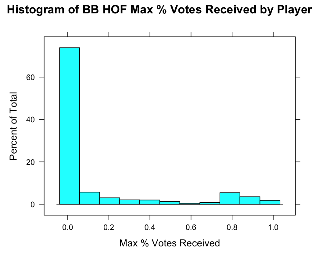
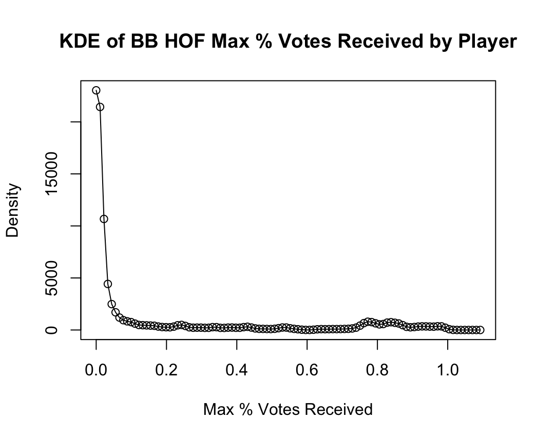
Figures 1a and 1b show histograms and kernel density estimates for max_pct. Note that kernel density estimates are computed with a Gaussian kernel and bandwidth set to the value given by Silverman’s rule of thumb, \(bw(X) = \frac{0.9}{n^{\frac{1}{5}}}\min\left({\sqrt{Var(x)}},{\frac{IQR(X)}{1.349}}\right)\)

The charts match our intuition – the majority of players receive close to no votes for the HOF, and interestingly even fewer players ever receive max votes in the 60-70% range. After 75% there appears more mass in the distribution, corresponding to the players who do successfully get in.

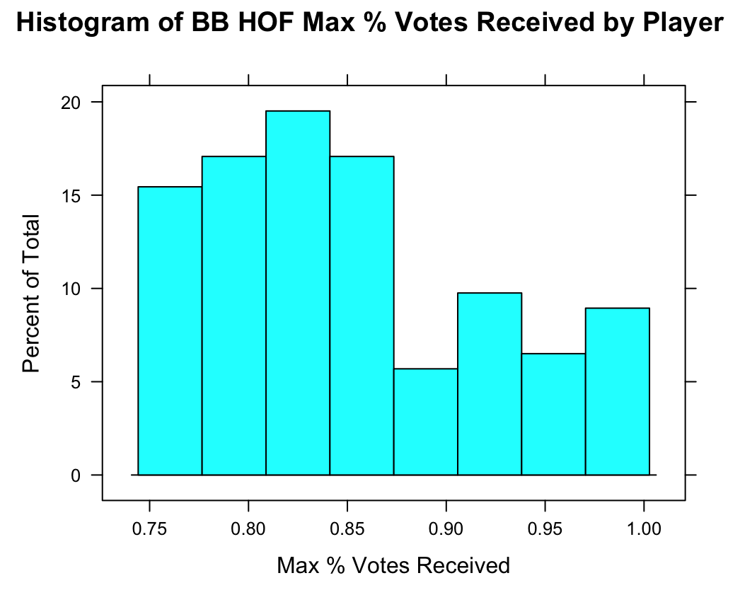
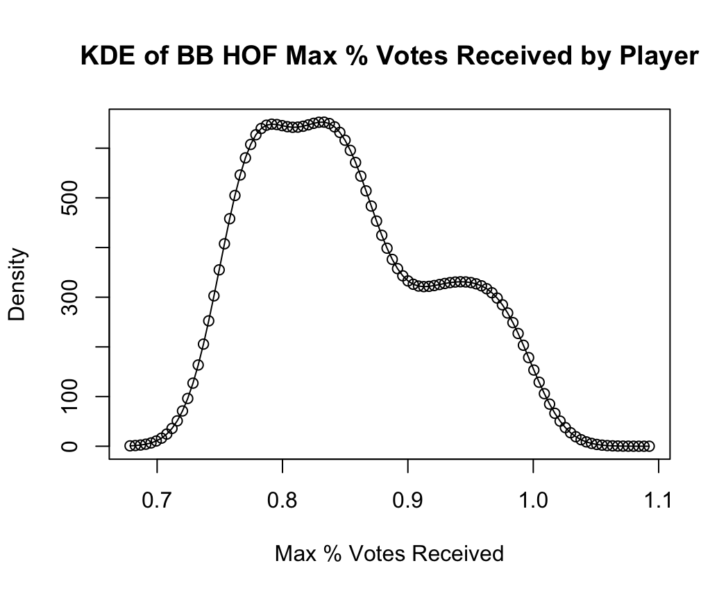
In Figure 2, we zoom in on the distribution of successful inductees’ max_pct. It’s most common for successful inductees to earn about 80% of the vote. We can visualize in the kernel density estimate the fact noted above that only one person ever has been elected unanimously, i.e., with 100% of the vote (a few others have received >98%!).

Predicting max_pct

With the above in mind, we fit a linear model for max_pct against our career batting data as covariates. The model summary can be found in Figure 3. All the batting variables are found to be significant to the 0.0001 level. The equation to estimate $\hat{\text{max_pct}}$ is given by

However, we note that the residuals of this model exhibit quite differently to what we would expect under standard homoscedasticity assumptions. The residuals vs fitted and normal Q-Q plots are depicted in Figure 4. With such uneven residual plots, we conclude that linear models may not be well suited to prediction of the max_pct variable.

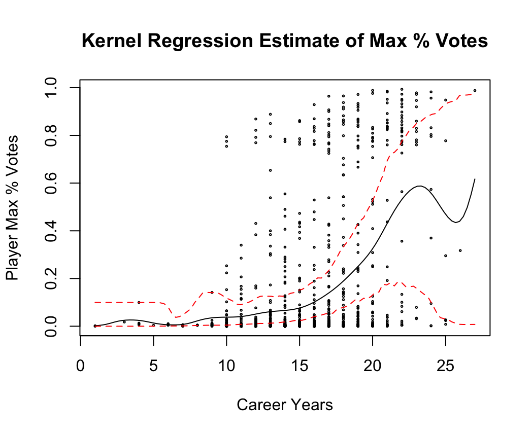
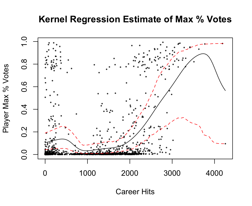
We attempt another regression analysis by performing kernel regressions against two of the career batting covariates. The results are shown in Figure 5. We also include 95% confidence intervals for the point estimates produced by the kernel regression.

Idiosyncrasies of the history of baseball may contribute to the wide CIs seen towards the upper end of the range for both covariates analyzed. As a case in point, there is one player who had on the order of 4000 hits represented in the Career Batting data set – this is Pete Rose, an outfielder who helped lead several Cincinnati Reds teams to successful seasons in the 1970s. He holds MLB records in many other batting statistics, including at-bats and games played. In 1989, Rose was discovered to have been gambling on the outcome of games he played in and managed, earning as a result a lifetime ban from professional baseball activity. He has never been elected to the Hall of Fame and likely will never be.

Classifying HOF Induction Status

We turn now to the second problem posed in the introduction, that of using machine learning algorithms to predict HOF induction status based on a given vector of career batting totals.

We generate train and test sets using the Career Batting dataset and evaluate four different approaches: quadratic discriminant analysis, logistic regression, and regression trees with and without cross-validation. Accuracy results for the four approaches are presented in Figure 6.

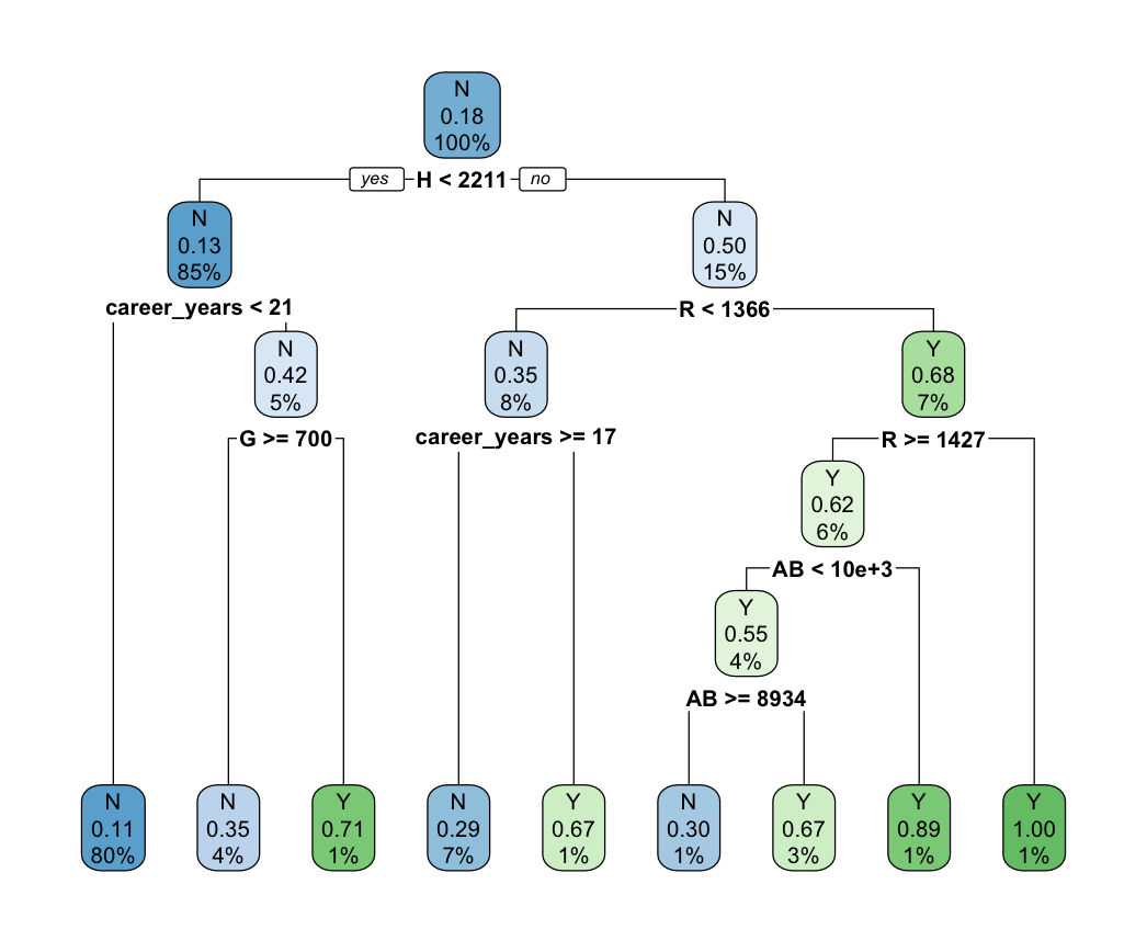
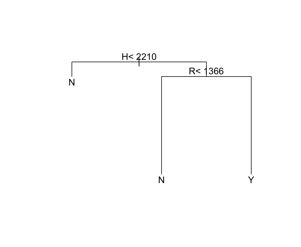
Overall, machine learning approaches are highly effective in the HOF induction problem, earning about 80% accuracy across the methods. For illustration’s sake, we depict in Figure 7 the branching points of the regression tree analyses. The utility of the cross-validated regression tree is in the simple rules given for decision making – any batter with more than 2,210 hits and 1,366 runs has a good case for inclusion in the Baseball Hall of Fame.

Challenges and Limitations

In the above report, we explore the application of statistical computing techniques to the question of analyzing data relating to induction into the Baseball Hall of Fame. While linear and kernel regression techniques come up short, we find that machine learning methods are highly applicable to the classification problem and can achieve 80% accuracy without much fine-tuning.

There were of course limitations to our approach. By only using Career Batting data, we ignore the fact that both batters and pitchers are included in the Hall of Fame. Any future work should seek to fold pitching data, which is comprised of variables distinct from those important in batting data, into the models used to predict or classify.

Another limitation is historical. Some of the greatest baseball players from a statistical standpoint were caught up in the steroid scandal of the late 1990s and early 2000s. Figures such as Barry Bonds, Mark McGwire, and Sammy Sosa rewrote batting statistics records playing under the influence of performance enhancing drugs and, as such, have effectively been shadowbanned from consideration for inclusion in the HOF. This is difficult for techniques which only have insight into the batting totals to identify a priori.

Figures

(Figure 1) Histogram and KDE for All Players

• (a) Histogram
• (b) KDE

(Figure 2) Histogram and KDE for Successful Inductees

• (a) Histogram
• (b) KDE

(Figure 3) Linear model summary for max_pct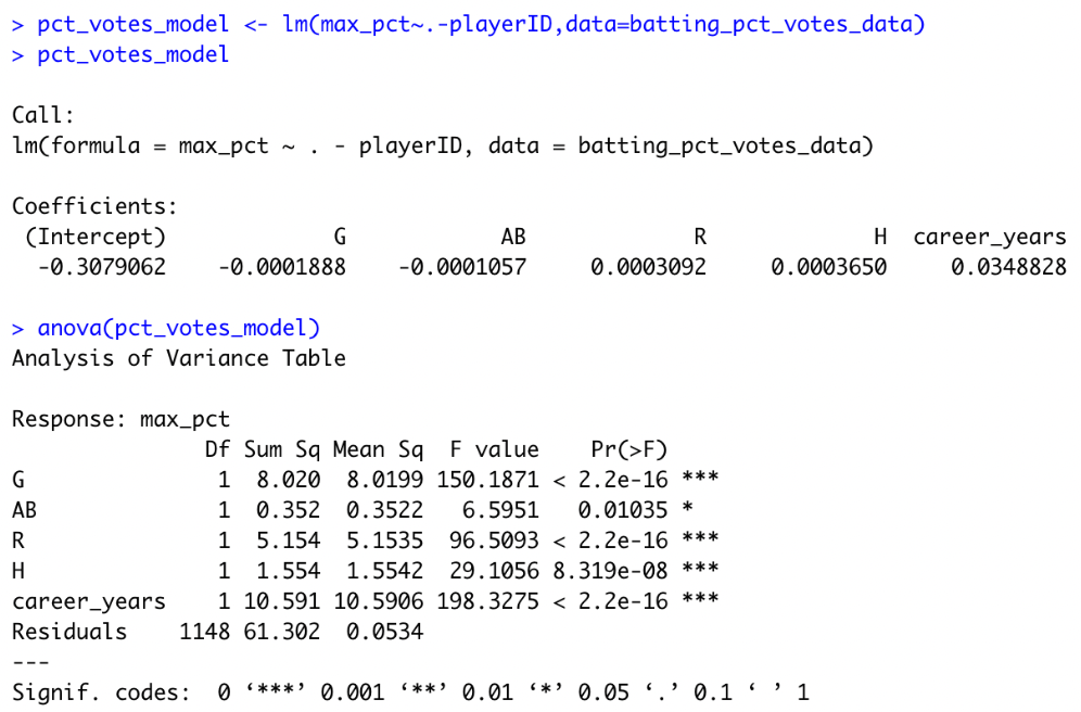

(Figure 4) Residual plots for linear model of max_pct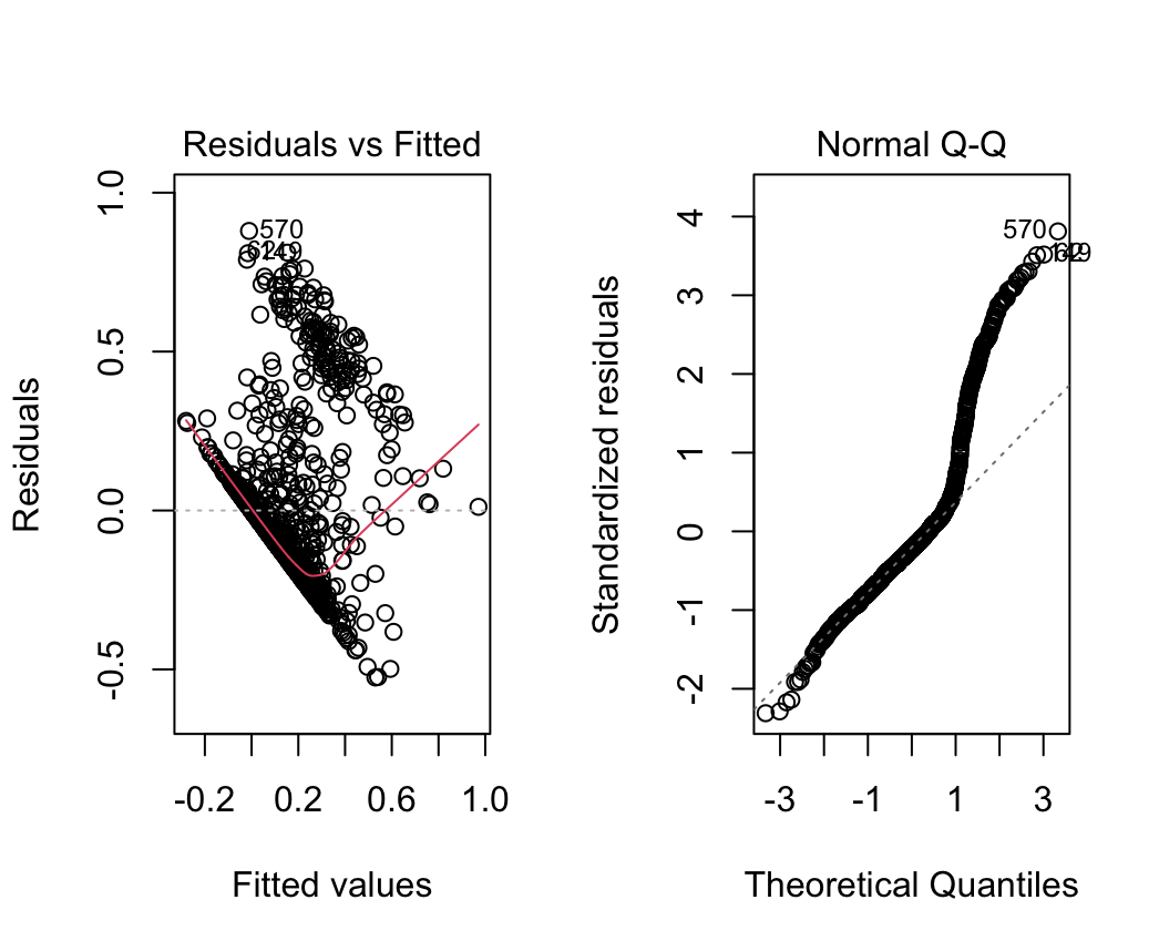

(Figure 5) Kernel Regression of max_pct Against Career Years and Hits

• (a) Kernel Regression vs Career Years
• (b) Kernel Regression vs Hits

(Figure 6) Accuracy from Confusion Matrices for Different ML Approaches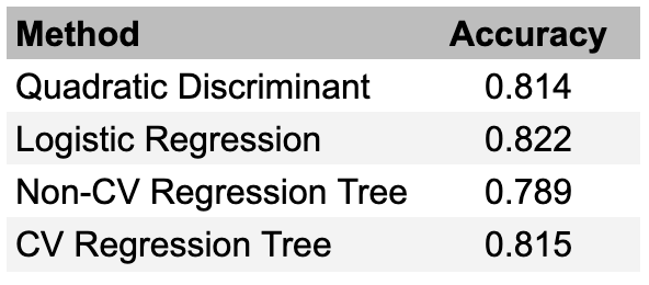

(Figure 7) Regression Tree Branching Points

• (a) Regression Tree 1
• (b) Regression Tree 2 (Cross-Validated)

Code

library(tidyverse)
library(XML)
library(RCurl)
library(rlist)
library(caret)
library(rpart)
library(rpart.plot)
system("R CMD SHLIB kernel.c")
dyn.load("kernel.so")
system("R CMD SHLIB kernreg.c")
dyn.load("kernreg.so")

### Data gathering and cleaning
## Reading in data from baseball_databank
theurl <- getURL("https://raw.githubusercontent.com/chadwickbureau/baseballdatabank/master/core/Batting.csv",.opts = list(ssl.verifypeer = FALSE))
tables <- read.csv(text=theurl)
batting_data <- tables

theurl <- getURL("https://raw.githubusercontent.com/chadwickbureau/baseballdatabank/master/core/People.csv",.opts = list(ssl.verifypeer = FALSE))
tables <- read.csv(text=theurl)
people_data <- tables

theurl <- getURL("https://raw.githubusercontent.com/chadwickbureau/baseballdatabank/master/contrib/HallOfFame.csv",.opts = list(ssl.verifypeer = FALSE))
tables <- read.csv(text=theurl)
hof_data <- tables

## Grouping and summarizing to get career batting totals
batting_totals <- batting_data %>% group_by(playerID) %>% mutate(career_years = n_distinct(yearID)) %>% summarize(G=sum(G),AB=sum(AB),R=sum(R),H=sum(H),career_years=max(career_years))
#eligible_batting_totals <- batting_totals %>% filter(career_years>=10)

## Grouping and summarizing to get max % votes won
max_vote_pct_by_player <- hof_data %>% filter(votedBy=='BBWAA') %>% mutate(pct_votes = votes/ballots) %>% group_by(playerID) %>% summarize(max_pct=max(pct_votes))
max_vote_pct_by_inductee <- max_vote_pct_by_player %>% filter(max_pct>0.75)

### Regression estimation section
## Histogram and kernel density estimation for % votes won
plot(density(max_vote_pct_by_player$max_pct))
histogram(max_vote_pct_by_player$max_pct,xlab='Max % Votes Received',main='Histogram of BB HOF Max % Votes Received by Player')
bw = bw.nrd0(max_vote_pct_by_player$max_pct)
grid <- seq(0.9*min(max_vote_pct_by_player$max_pct),1.1*max(max_vote_pct_by_player$max_pct),length.out=100)
y <- double(length(grid))
y_est <- .C("get_kernel_density",as.double(max_vote_pct_by_player$max_pct),as.integer(length(max_vote_pct_by_player$max_pct)),as.double(grid),as.integer(length(grid)),as.double(y),as.double(bw))
plot(grid,y_est[[5]],xlab='Max % Votes Received',ylab='Density',main='KDE of BB HOF Max % Votes Received by Player')
lines(grid,y_est[[5]])

## Histogram and kernel density estimation for % votes won inductees-only 
histogram(max_vote_pct_by_inductee$max_pct,xlab='Max % Votes Received',main='Histogram of BB HOF Max % Votes Received by Player')
bw = bw.nrd0(max_vote_pct_by_inductee$max_pct)
grid <- seq(0.9*min(max_vote_pct_by_inductee$max_pct),1.1*max(max_vote_pct_by_inductee$max_pct),length.out=100)
y <- double(length(grid))
y_est <- .C("get_kernel_density",as.double(max_vote_pct_by_inductee$max_pct),as.integer(length(max_vote_pct_by_inductee$max_pct)),as.double(grid),as.integer(length(grid)),as.double(y),as.double(bw))
par(mfrow=c(1,1))
plot(grid,y_est[[5]],xlab='Max % Votes Received',ylab='Density',main='KDE of BB HOF Max % Votes Received by Player')
lines(grid,y_est[[5]])

## Joining pct_votes and batting tables
batting_pct_votes_data <- batting_totals %>% right_join(max_vote_pct_by_player) %>% drop_na()

## Linear regression on % votes won
pct_votes_model <- lm((max_pct)~.-playerID,data=batting_pct_votes_data)
summary(pct_votes_model)
anova(pct_votes_model)
par(mfrow=c(1,2))
plot(pct_votes_model,which=c(1,2))

## Logistic regression on % votes won
batting_pct_votes_data_w_induction <- batting_pct_votes_data %>% mutate(inducted = case_when(max_pct >= 0.75 ~ 1, max_pct < 0.75 ~ 0))
pct_votes_model_logit <- glm(inducted~.-playerID-max_pct,data=batting_pct_votes_data_w_induction,family='binomial')
summary(pct_votes_model_logit)
anova(pct_votes_model_logit)
plot(pct_votes_model_logit)

## Kernel regressions
# Pct ~ years
par(mfrow=c(1,1))
x <- batting_pct_votes_data$career_years
y <- batting_pct_votes_data$max_pct
b <- bw.nrd(x)
x_grid <- as.double(seq(min(x),max(x),length=100))
grid_length <- 100
results_grid <- double(100)
length_x <- length(x)
a <- .C("kernreg",as.double(x),as.double(y),as.integer(length_x),as.double(b),as.double(x_grid),as.integer(grid_length),as.double(results_grid))
plot(c(min(x),max(x)),c(min(y),max(y)),xlab="Career Years",ylab='Max % Votes',main='Kernel Regression of Max % Votes on Career Years')
lines(a[[5]],a[[7]])
points(a[[1]],a[[2]])

sample_df <- as.data.frame(cbind(x,y))
results_df <- data.frame(matrix(ncol=200,nrow=100))
i=1
while(i <= 200){
  temp <- sample_n(sample_df,100,replace=TRUE)
  new_x <- temp$x
  new_y <- temp$y
  a_temp <- .C("kernreg",as.double(new_x),as.double(new_y),as.integer(length(new_x)),as.double(b),as.double(x_grid),as.integer(grid_length),as.double(double(grid_length)))
  results_df[i] <- a_temp[[7]]
  i <- i + 1
}

low_CI <- double(nrow(results_df))
hi_CI <- double(nrow(results_df))
for(i in 1:nrow(results_df)){
  low_CI[i] <- sort(results_df[i,])[5]
  hi_CI[i] <- sort(results_df[i,])[195]
}

sort(results_df[2,])[3]
sort(results_df[2,])[97]
plot(c(min(x),max(x)),c(min(y),max(y)),type='n',main='Kernel Regression Estimate of Max % Votes',ylab='Player Max % Votes',xlab='Career Years')
points(a[[1]],a[[2]],cex=0.25)
lines(a[[5]],a[[7]])
lines(a[[5]],low_CI,lty=2,col='red')
lines(a[[5]],hi_CI,lty=2,col='red')

# Pct ~ hits
x <- batting_pct_votes_data$H
y <- batting_pct_votes_data$max_pct
b <- bw.nrd(x)
x_grid <- as.double(seq(min(x),max(x),length=100))
grid_length <- 100
results_grid <- double(100)
length_x <- length(x)
a <- .C("kernreg",as.double(x),as.double(y),as.integer(length_x),as.double(b),as.double(x_grid),as.integer(grid_length),as.double(results_grid))
plot(c(min(x),max(x)),c(min(y),max(y)),xlab="Career Hits",ylab='Max % Votes',main='Kernel Regression of Max % Votes on Career Hits')
lines(a[[5]],a[[7]])
points(a[[1]],a[[2]])

sample_df <- as.data.frame(cbind(x,y))
results_df <- data.frame(matrix(ncol=200,nrow=100))
i=1
while(i <= 200){
  temp <- sample_n(sample_df,100,replace=TRUE)
  new_x <- temp$x
  new_y <- temp$y
  a_temp <- .C("kernreg",as.double(new_x),as.double(new_y),as.integer(length(new_x)),as.double(b),as.double(x_grid),as.integer(grid_length),as.double(double(grid_length)))
  results_df[i] <- a_temp[[7]]
  i <- i + 1
}

low_CI <- double(nrow(results_df))
hi_CI <- double(nrow(results_df))
for(i in 1:nrow(results_df)){
  low_CI[i] <- sort(results_df[i,])[5]
  hi_CI[i] <- sort(results_df[i,])[195]
}

sort(results_df[2,])[3]
sort(results_df[2,])[97]
plot(c(min(x),max(x)),c(min(y),max(y)),type='n',main='Kernel Regression Estimate of Max % Votes',ylab='Player Max % Votes',xlab='Career Hits')
points(a[[1]],a[[2]],cex=0.25)
lines(a[[5]],a[[7]])
lines(a[[5]],low_CI,lty=2,col='red')
lines(a[[5]],hi_CI,lty=2,col='red')

### Classification section
## Joining onto HOF table
hof_data <- hof_data %>% distinct(playerID,inducted)
batting_hof_data <- batting_totals %>% right_join(hof_data) %>% drop_na()

## Just doing a nice plot
batting_hof_data  %>% ggplot(aes(H, career_years, fill = inducted, color=inducted)) +
  geom_point(show.legend = FALSE) +
  stat_ellipse(type="norm") 

## Generating train set/test set
y <- batting_hof_data$inducted
test_index <- createDataPartition(y, times = 1, p = 0.5, list=F)
train_set <- batting_hof_data %>% slice(-test_index)
test_set <- batting_hof_data %>% slice(test_index)

## QDA model
params <- train_set %>% group_by(inducted) %>% summarise(avg1=mean(R,na.rm=T),sd1=sd(R,na.rm=T),avg2=mean(career_years,na.rm=T),sd2=sd(career_years,na.rm=T),r=cor(R, career_years,use="complete.obs"))
train_qda <- train(inducted~R+H+G+AB+career_years,method="qda",data=train_set)
y_hat <- predict(train_qda,test_set)
confusionMatrix(y_hat,as.factor(test_set$inducted))$overall['Accuracy']

## Logistic model
train_logistic <- glm(as.factor(inducted)~R+H+G+AB+career_years, data=train_set,family="binomial")
p_hat_logit <- predict(train_logistic, newdata = test_set, type = "response")
y_hat_logit <- ifelse(p_hat_logit > 0.5, "Y", "N") %>% factor()
confusionMatrix(y_hat_logit, as.factor(test_set$inducted))$overall["Accuracy"]

## Classification tree with rpart and cross-validation
# Non-CV tree
par(mfrow=c(1,1))
train_rpart <- rpart(as.factor(inducted)~R+H+G+AB+career_years, data=train_set)
rpart.plot(train_rpart)
summary(train_rpart)
y_hat_naive <- predict(train_rpart,test_set,type="class")
confusionMatrix(y_hat_naive,as.factor(test_set$inducted))$overall['Accuracy']

# CV tree
train_rpart_fit <- train(as.factor(inducted)~R+H+G+AB+career_years, data=train_set,method='rpart',tuneGrid=data.frame(cp = seq(0.0, 0.1, len = 25)))
ggplot(train_rpart_fit)
plot(train_rpart_fit$finalModel,margin=0.1)
text(train_rpart_fit$finalModel)
y_hat <- predict(train_rpart_fit,test_set)
confusionMatrix(y_hat,as.factor(test_set$inducted))$overall['Accuracy']

### Predicting 2023 1st time ballot
first_timers_2023 = c('Bronson Arroyo','Carlos Beltran','Matt Cain','R.A. Dickey','Jacoby Ellsbury','Andre Ethier','J.J. Hardy','John Lackey','Mike Napoli','Jhonny Peralta','Francisco Rodríguez','Huston Street','Jered Weaver','Jayson Werth')
first_timers_2023_people <- people_data %>% mutate(fullName = paste(nameFirst, nameLast)) %>% filter(fullName %in% first_timers_2023)
first_timers_2023_batting <- batting_data %>% group_by(playerID) %>% mutate(career_years = n_distinct(yearID)) %>% summarize(G=sum(G),AB=sum(AB),R=sum(R),H=sum(H),career_years=max(career_years)) %>% right_join(first_timers_2023_people) %>% select(playerID,G,AB,R,H,career_years)
predict(train_rpart,first_timers_2023_batting)


mcgriff_stats <- people_data %>% mutate(fullName = paste(nameFirst, nameLast)) %>% filter(fullName =='Fred McGriff')
mfgriff_batting <- batting_data %>% group_by(playerID) %>% mutate(career_years = n_distinct(yearID)) %>% summarize(G=sum(G),AB=sum(AB),R=sum(R),H=sum(H),career_years=max(career_years)) %>% right_join(mcgriff_stats) %>% select(playerID,G,AB,R,H,career_years) %>% mutate(inducted='N')
predict(train_rpart,mfgriff_batting)

ramirez_stats <- people_data %>% mutate(fullName = paste(nameFirst, nameLast)) %>% filter(fullName =='Manny Ramirez')
ramirez_batting <- batting_data %>% group_by(playerID) %>% mutate(career_years = n_distinct(yearID)) %>% summarize(G=sum(G),AB=sum(AB),R=sum(R),H=sum(H),career_years=max(career_years)) %>% right_join(mcgriff_stats) %>% select(playerID,G,AB,R,H,career_years)
predict(train_rpart,ramirez_batting)